Planning Mode

Planning mode starts with the agent generating an “Implementation Plan” and asking for approval before proceeding. You can comment on the plan and have AI iterate on it until you’re ready to proceed. The Antigravity interface for reviewing the plan is great and being able to comment on individual plan items works well for making minor changes to the overall plan. The produced plan follows a general structure of “Proposed Changes”, broken down into “Structure” and “Components”, and then “Verification Plan”, broken down into “Automated Tests” and “Manual Verification”. I prefer to see the updated plan after leaving comments but sometimes AI feels confident enough to proceed without showing me the updated plan. I’ve found Claude and Gemini 3 Flash to be more eager to proceed compared to Gemini 3/3.1 Pro.

Typically my comments are bike-shedding about names of functions or files but occasionally I’ll have more substantial comments about the implementation of an API or database schema. This is especially true when decisions require context about the larger vision of the project or future features that could be added.

Review

As the agent completes its tasks, it starts to show a list of “artifacts” which are files in the repo that were changed thus far. The artifacts list is shared between agents so it can be confusing at times why certain files are showing up. However, it’s helpful to see what’s being changed and you can start to review the changes per-file. There’s also an “Accept All” button if you are comfortable with all of the changes and don’t need to review each one.

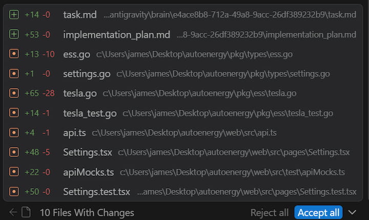
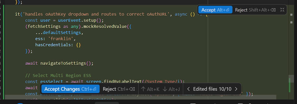
Once the agent has completed all the tasks it generates a “Walkthrough” that explains all the changes it made. I rarely find this useful and instead start to just review the files changed. Each file changed is shown in the agent window and you can click through to see the diff right in the editor. You can accept or reject chunks of changes, all changes in the file, or all changes in the project. This is the best interface I’ve used for reviewing changes and I prefer being able to review them immediately right in the editor compared to pushing and reviewing in the PR.

Models

Despite paying for Google’s AI Pro plan ($20/mo) I regularly hit the Gemini 3.1 Pro rate limit and that used to just mean a 5 hour cooldown. I’d go to bed and in the morning have a fresh slate. However, as of a few weeks ago the Pro models have a 7 day cooldown. As a result, I rarely end up using the Pro models except for very specific difficult features or for planning. I’ve tried Sonnet 4.6 and Opus 4.6 numerous times but haven’t seen a significant improvement. However, they’ve proven useful for reviews and double-checking the work of myself or another model.

Gemini 3 Flash is now my go-to model for most tasks. It’s fast and does a good job at simple Go and React coding. I have to usually critique its changes but overall it’s still much faster than writing all of the code myself. Tests are the area I want to use it the most but I’ve found it to do a poor job at writing comprehensive tests that include several assertions. For example, it loves to use mock.Anything for all of the arguments in mocks rather than specifically asserting the significant values. I haven’t yet found a way to consistently get it to write comprehensive tests in the format I expect. It also struggles with debugging failing tests and sometimes alters code to fix a failing test rather than correcting the test.

Commands

The agent can run commands to lint files, execute tests, install dependencies, and more. The agent by default requests review before every command but you can configure it to always proceed with any command (YOLO-style). Since reviewing every command can be tedious there’s an allow list and a deny list, which theoretically should cover the majority of commands. My allow list contains things like go test, npm run test, npm run build, ls, grep and these are supposed to match command prefixes but I’ve found it to only work half the time. 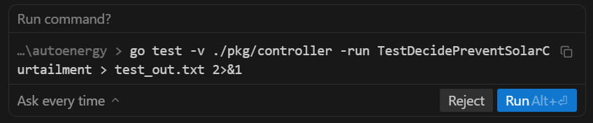For example, the agent asked to run the following command even though go test is in my allow list. I haven’t figured out exactly why but I think it has to do with it redirecting the output. Commands that contain a pipe | trigger it as well even if it’s in a string.

Autocomplete

The autocomplete in Antigravity generally predicts up to a few lines ahead and will not autocomplete whole functions or blocks of code in one tab. Cursor’s autocomplete was way too eager and I would often accidentally accept autocomplete changes when indenting code. The biggest benefit I get from autocomplete are making several similar consecutive changes like adding an argument to a method or refactoring a common line of code. It’s convenient to be able to tab though the file tweaking each spot.

I use the Go LSP server and commonly find Antigravity’s autocomplete competing and less useful than the native Go extension’s autocomplete when I’m trying to call a method, access a field, or start a callback signature. Go has the advantage of knowing the names of things that don’t exist in the current file or even the repo. This was frustrating even when I was using Cursor so I don’t expect it to be easy to solve.

Multiple Agents

Antigravity supports concurrent agents within or across repositories. The agent manager window gives you an overview of all active chats across repositories. Given how closely I monitor and review the agent’s work, I haven’t found myself orchestrating multiple agents across repositories yet. I seldom have concurrent chats going on within a project because they tend to step on each other’s toes especially when debugging tests. If I can ensure a clear separation of work, like different packages or folders, then it has come in handy. As the agents improve and they can operate independently for longer, I see myself utilizing this feature more.

Final Verdict

Overall I’ve been more productive using Antigravity compared to without it despite some of the frustrations I shared. It’s only been out for a few months and during that time I haven’t seen it change much outside of the availability of the models. I’m looking forward to Google addressing some of the issues.

BigQuery tables can be partitioned and clustered. Partitions divide your data into integer-based or date-based blocks colocating in storage with the same values. Clustering further sorts the rows within those partitions by the specified columns. Partitioning and clustering can be used to significantly optimize query performance by reducing how much data is processed when the queries filter on those columns. Keep in mind that the BigQuery bytes estimate for a query takes into account partitioning but not always clustering.

Table sampling works by selecting a subset of the data blocks necessary for a given query. So a table sample of 50 percent will roughly read half of the data blocks, assuming the table is sufficiently large and has many data blocks.

Examples

Let’s look at some examples of queries that use all three techniques using the pageview_2025 table of the public wikipedia dataset.

The first query simply counts how many rows are in the table but this requires reading over 800GB of data. That’s pretty inefficient and in fact, this table is configured with a required partition filter, so you can’t even run this query. If you could, it would return 158,583,259,826 views.

SELECT SUM(views)
FROM `bigquery-public-data.wikipedia.pageviews_2025`

Let’s reduce the number of partitions by including a WHERE clause on the datehour column to limit the rows to only those in October and switch to getting the total pageviews. This query reads only 72GB of data, processing 4,876,284,775 rows for a total of 14,445,367,832 views.

...
WHERE TIMESTAMP_TRUNC(datehour, DAY) >= "2025-10-01"
  AND TIMESTAMP_TRUNC(datehour, DAY) < "2025-11-01"

This table is also clustered by the wiki (subdomain) and title columns to allow for efficient pageview counts by page and domain. If we also filter on wiki (one of the clustering columns) in our query we will further reduce the data that’s read. This query only reads 6GB of data and it returns 267,013,325.

...
  AND wiki = 'de'

We could sample on a per-row basis using RAND() and BigQuery would have to read all of the data. We just determined that was 6GB and this query returns 26,494,288 (your results may vary).

...
  AND RAND() < 0.1

In contrast, if we use TABLESAMPLE to add sampling of 10 percent, full query shown below, BigQuery will roughly read a tenth of the data blocks. The following query reads only 544MB of data.

SELECT SUM(views)
FROM `bigquery-public-data.wikipedia.pageviews_2025`
TABLESAMPLE SYSTEM (10 PERCENT)
WHERE TIMESTAMP_TRUNC(datehour, DAY) >= TIMESTAMP("2025-10-01")
  AND TIMESTAMP_TRUNC(datehour, DAY) < TIMESTAMP("2025-11-01")
  AND wiki = 'de'

Let’s run that query 10 times:

Notice the massive variance, ranging from 9 million to over 30 million views. The total views was 267 million so we would’ve expected around 26 million as a result and we only got close to that result twice.

Sampling Bias

The pageview data for October contains 1,980 distinct wiki values and 238,667,980 distinct title values. Remember that clustering sorts similar rows together in data blocks and table sampling will limit the query to a subset of those blocks. As we just saw, this can lead to sampling bias if the features are used together for a query. The last query looks at only a tenth of the blocks and depending on which titles and which times are included in those blocks you get vastly different answers.

For a given hour in October for the de wiki gets between approximately 52,000 views and 897,000 views with the following distribution:

However the distribution of views by title is heavily skewed towards the homepage, which received 15,755,415 pageviews. The 90th percentile was a mere 48 pageviews.

Because table sampling works at the block-level, the results are a lottery. If your sample happens to include some homepage blocks, you’ll get a large number otherwise it’ll be far too low.

I’m glad to see that Google finally acknowledges this and added a section outlining how it performs on partitioned and clustered tables to the documentation. However, it should be much more prominent or the feature should consider being removed completely. If you’re considering table sampling you probably have a large table and if you have a large table you should be using partitions and/or clustering.

The bias is most extreme when you have clustered data that is not evenly distributed or when you’re using a small sample size. You can stick to using RAND() your data isn’t suitable for TABLESAMPLE, especially for one-off queries. But if you have a constant need for sampled data your archicture allows for it, instead sample the data outside of BigQuery and write to a separate “sample” table during insertion.

Note: BigQuery does not support the BERNOULLI sampling method.

In Go 1.21, the ParseIP method was changed (and later documented) to always return a 16-byte IP, representing IPv4 addresses as IPv4-mapped IPv6 addresses. The net package treats IPv4-mapped IPv6 addresses and IPv4 addresses as equivalent, so this change should not have altered behavior.

However, Contains always calls To4 on the provided IP:

if x := ip.To4(); x != nil {
  ip = x
}

This call previously did nothing for IPv4 addresses, but now it ends up slicing the IP whenever it’s an IPv4-mapped IPv6 address (which, after the 1.21 change, is all the time for IPv4 addresses).

func (ip IP) To4() IP {
	if len(ip) == IPv4len {
		return ip
	}
	if len(ip) == IPv6len &&
		isZeros(ip[0:10]) &&
		ip[10] == 0xff &&
		ip[11] == 0xff {
		return ip[12:16]
	}
	return nil
}

The conversion from IPv4-mapped to IPv4 is only a couple nanoseconds slower

BenchmarkContainsV4-16                    88157508             12.51 ns/op
BenchmarkContainsV4Mapped-16              64967758             20.06 ns/op
BenchmarkContainsV6-16                    89194792             12.97 ns/op

which is insignificant unless you’re checking if an IP is contained against a list of 1,000 networks.

BenchmarkContainsV4List-16                  148334              7111 ns/op
BenchmarkContainsV4MappedList-16             90250             13092 ns/op
BenchmarkContainsV6List-16                  153919              7656 ns/op

This was discovered during an investigation into an increase in CPU usage affecting certain servers in our fleet. On some servers, Contains accounted for more than 30% of CPU time and a 7x increase in time spent running the garbage collector. The difference between servers was related to the proportion of IPv4 vs IPv6 addresses that the server was handling.

Solution 1: Custom Contains

After we narrowed the problem down to the To4 method my first attempt at a solution was to write a custom function that checked for IPv4-mapped IPv6 addresses and handled them separately by checking the mask against the last 4 bytes without reslicing the IP. This solution reduced the time by more than 50%.

func Contains(ipn *net.IPNet, ip net.IP) bool {
	// explicitly check for ipv4-mapped ipv6 addresses
	if len(ip) == net.IPv6len && bytes.HasPrefix(ip, v4InV6PrefixBytes) {
		// make sure ipnet is an ipv4 address
		if len(ipn.IP) != net.IPv4len {
			return false
		}
		// we only look at bytes 12 though 16
		for i := range ipn.IP {
			if ipn.IP[i] != ip[i+12]&ipn.Mask[i] {
				return false
			}
		}
		return true
	}
	if len(ipn.IP) != len(ip) {
		return false
	}
	for i := range ipn.IP {
		if ipn.IP[i] != ip[i]&ipn.Mask[i] {
			return false
		}
	}
	return true
}

BenchmarkCustomContainsV4List-16             377374            3093 ns/op
BenchmarkCustomContainsV4MappedList-16       183717            5904 ns/op
BenchmarkCustomContainsV6-16                 174031            6102 ns/op

This restored stability to the service and reduced the CPU usage, but there was still a large discrepancy between servers, and as the list of networks we checked against grew, the difference became more pronounced.

Solution 2: Optimized Lookups

As I worked to improve the performance further I tried several things. First, I should store the IPv4 and IPv6 networks separately and only check against the relevant list. Second, I could swap bytes.HasPrefix for a string comparison when determining if an IP is an IPv4-mapped IPv6 address. Finally, I can use the prefix from the network as a key in a map to further reduce the number of comparisons needed.

This resulted in something similar to:

type IPNetSet struct {
	m4 map[string][]*net.IPNet
	m6 map[string][]*net.IPNet
}

// Find returns the first IPNet that contains the given ip.
func (s *IPNetSet) Find(ip net.IP) (*net.IPNet, bool) {
	switch {
	case len(ip) == net.IPv4len:
		for _, e := range s.m4[string(ip[:1])] {
			if Contains(e, ip) {
				return e, true
			}
		}
	case len(ip) == net.IPv6len && string(ip[:12]) == v4InV6Prefix:
		ip = ip[12:]
		for _, e := range s.m4[string(ip[:1])] {
			if Contains(e, ip) {
				return e, true
			}
		}
	case len(ip) == net.IPv6len:
		for _, e := range s.m6[string(ip[:2])] {
			if Contains(e, ip) {
				return e, true
			}
		}
	}
	return nil, false
}

With this solution, the time was reduced by almost 100x. The IP network lookups now barely register in CPU usage and we can handle orders of magnitude more networks if we had to. Additionally, there’s almost no difference between the different forms of IPv4 IPs.

BenchmarkMapContainsV4List-16               41507410         28.53 ns/op
BenchmarkMapContainsV4MappedList-16         43106853         28.75 ns/op
BenchmarkMapContainsV6-16                   33591614         32.12 ns/op

Further Optimizations

Currently, the map key only contains the first byte of IPv4 and the first 2 bytes of IPv6 networks. The sweet spot largely depends on the distribution of the networks and what your maximum mask is. I’ll likely explore tweaking these further. But for now, the performance is good enough that I have more important things to focus on.

The rest of the codebase used net.IP and switching everything over to the new net/netip package would’ve been more work than I was willing to do at the time. I’ll be exploring this further in the future as we move to netip in general. I did benchmark the netip.Prefix method and it was much faster than net.IPNet along with no difference between the different IP versions.

BenchmarkNetIPContainsV4List-16             275042          4318 ns/op
BenchmarkNetIPContainsV4MappedList-16       269730          4592 ns/op
BenchmarkNetIPContainsV6List-16             239674          4715 ns/op

The code and benchmarks above can be found in 2025-go-ipnet-improvements.